Subnational microsimulation needs survey microdata that reproduce administrative totals across nested geographies while staying usable inside a policy model. A fidelity-oriented pipeline can combine many sources and add record-level variation, producing a candidate dataset rich enough to represent the targets but too large to simulate. That dataset has to be reduced, and the question is which records to keep.
We study this reduction as a sampling problem. Using \(L_0\) regularization with the Hard Concrete relaxation of Louizos et al. (2018), the method jointly selects which records to retain and assigns each a positive weight, with selection driven by the calibration targets rather than drawn at random. The gates make the retained-record count an explicit optimization variable, and soft and hard concentration controls bound how large individual weights can grow. Because the optimization that selects records also calibrates them, the reduced dataset continues to match its targets.
We implement the method within Populace, PolicyEngine’s microsimulation data pipeline, and present a proof of concept on its current full United States target surface. The run starts from 37,053 Ledger facts and scores 32,633 materialized calibration targets, including 24,340 congressional-district targets, on 337,704 candidate households from a three-year pooled ASEC support file. Holding the candidate universe, target surface, and optimizer budget fixed, we vary how records are chosen across target-informed \(L_0\) selection, dense no-\(L_0\) calibration, and matched sampling baselines, all scored by the same Populace capped weighted calibration loss. A normalized \(L_0\) penalty retaining 57,240 records produces a sparse support whose raw gated weights score poorly, but an ordinary post-\(L_0\) refit on that support lowers the Populace loss to 4.74%. The 1,500-epoch dense no-\(L_0\) calibration reaches 5.07%, a random subset followed by the same reweighting reaches 7.55%, and a random sample of the dense calibrated weights scaled back to total mass reaches 24.24%. The useful finding is therefore specific and actionable: the gates are valuable as a support selector, while the publication weights should be refit after selection. Because the dense loss is still declining at the endpoint, the result is a finite-optimization and sparse support result rather than a claim that dense calibration could not converge lower. The machinery now runs the full surface, preserves the resulting weight vectors, and sets up the next robustness work: normalized-penalty sweeps, longer dense convergence checks, concentration controls, and comparisons against classical calibration methods on target subsets where their assumptions hold.
Keywords: microsimulation, survey calibration, subsampling, \(L_0\) regularization, subnational analysis
Tax-benefit microsimulation models apply policy rules to household microdata to estimate fiscal and distributional effects. At the national level, that usually means starting from a survey such as the Current Population Survey (CPS), improving measured incomes and program participation, and adjusting weights so the dataset reproduces known aggregates. Subnational work is harder. Analysts often want estimates for states, congressional districts, or local areas, but the underlying survey was not designed to support all of those geographies at once.
That gap matters in practice, because many reforms are proposed, administered, or debated below the national level. A state tax proposal needs state-specific incomes, filing patterns, and benefit participation. District-level analysis needs those same outcomes to aggregate correctly within each district while staying consistent with state and national totals. A usable subnational dataset therefore has to satisfy a hierarchical calibration problem rather than a single national one.
One way to meet that demand is to build a dataset that carries as much of the relevant variation as possible. A pipeline can combine several surveys and administrative files, impute the variables that any single source lacks, and attach the geographic detail that local analysis needs. Each of these steps enriches the records, and some add records. The result is a candidate dataset rich enough to represent the variation the targets describe, and large enough that it becomes expensive to store, calibrate, and simulate. A file with millions of active records supports detailed subnational work but is slow to run; a much smaller file is easier to ship, but only if the loss in fidelity is acceptable.
The candidate dataset therefore has to be reduced to a size that can be shipped and simulated, and this paper treats that reduction as a sampling problem: given the large candidate universe and a fixed record budget, which records should the final dataset keep, and what weight should each kept record carry? The simplest answer is to draw a random subset and reweight it to the targets. We study an alternative in which the selection itself is informed by the targets.
The method is \(L_0\) regularization with the Hard Concrete relaxation (Louizos et al. 2018). Each candidate record receives a gate that the optimizer can drive toward zero or one, and the expected number of open gates enters the objective directly. Minimizing calibration error and the gate count together selects a subset of records and fits their weights in one optimization. The retained-record count becomes a quantity the optimizer controls rather than a fixed draw, and two concentration controls (a soft penalty and a hard per-record cap) limit how concentrated the fitted weights can become. In practical terms, one framework can target a compact national dataset or a larger subnational dataset, at a chosen record budget, with weights kept inside a usable range.
We situate this work in Populace (PolicyEngine 2026b), PolicyEngine’s pipeline for microsimulation dataset construction. Populace passes a single weighted data structure through a sequence of modular stages—source loading, imputation, geographic assignment, target construction, and calibration—each implemented as a separate package operating on that shared structure. Because the stages are modular, the data sources, the imputation model, the geographic assignment, and the calibration method are interchangeable components rather than fixed code, and the calibration step studied here is one such component. The paper describes the pipeline at the level needed to follow the calibration step, and then describes the configuration used here.
This paper is a proof of concept on Populace’s current full target surface: it asks whether \(L_0\) selection with Hard Concrete gates can produce a sparse, calibrated dataset on the targets Populace assembles today, including the congressional-district surface that motivates the build-big, then-prune workflow. Local-area and subnational calibration are therefore part of the target surface being fit, while full production release engineering remains outside the scope of the proof of concept.
The empirical question is whether informed selection earns its added complexity. We ask three things. First, on the actual Populace loss over the full target surface, does informed \(L_0\) selection or its post-\(L_0\) refit reproduce the targets more accurately than dense calibration and sampling baselines under the same optimizer budget? Second, what do supplemental raw-error diagnostics reveal about the tail of the target distribution? Third, does the framework give usable control over the size of the output and the concentration of the fitted weights? The current full-surface probe gives a constructive answer: the raw gated \(L_0\) weights are not good enough by themselves, but the support selected by the gates becomes more accurate than matched random support and slightly lower-loss than the 1,500-epoch dense no-\(L_0\) run after an ordinary calibration refit.
The rest of the paper follows that structure. Section 2 places the work in the literature on spatial microsimulation, survey calibration, and sparse selection. Section 3 describes the base microdata, the Populace pipeline, and the administrative targets. Section 4 presents the calibration method and the sampling experiment design. Section 5 reports the comparison against the sampling baselines and the behaviour of the size, geography, and weight controls. Section 6 interprets those results and discusses their limits, and Section 8 concludes.
Subnational microsimulation starts from a recurring problem: a national survey carries the behavioural and demographic detail needed for policy modelling, but it does not contain enough observations in every local area to support direct estimation. Spatial microsimulation addresses that gap either by reweighting existing survey records or by building synthetic small-area populations from aggregate constraints (Tanton 2014; O’Donoghue et al. 2014).
This distinction matters for the present work, because our pipeline is a reweighting system built on observed CPS households. It places households across geographies to create local variants, but the core problem remains the calibration of survey-based microdata to administrative targets, which keeps calibration methods as the closest reference point.
The spatial microsimulation literature supplies further context. Williamson et al. (1998), Huang and Williamson (2001), and Harland et al. (2012) describe combinatorial and synthetic-population approaches that search over record assignments area by area. Tanton et al. (2011) and Lovelace and Dumont (2016) discuss reweighting for small-area estimation and policy analysis. These methods usually target one geographic layer at a time, whereas our setting asks one weighted dataset to reproduce state and national targets together.
Let \(i = 1, \ldots, n\) index sampled units, let \(d_i\) denote the initial design weight for unit \(i\), and let \(\mathbf{x}_i \in \mathbb{R}^p\) denote the auxiliary variables used for calibration. Survey calibration seeks adjusted weights \(w_i\) whose weighted totals match known population totals: \[\begin{equation} \sum_{i=1}^{n} w_i \mathbf{x}_i = \mathbf{T}, \label{eq:calibration_constraint} \end{equation}\] where \(\mathbf{T} \in \mathbb{R}^p\) is the vector of published totals (Deville and Särndal 1992; Särndal 2007). The auxiliary variables may be counts, indicators, or continuous quantities such as income components.
The subnational problem extends this setup in two ways. The target vector draws on several administrative sources, so it mixes count and dollar constraints. The constraints are also nested by geography: district totals should sum to state totals, which should sum to national totals after uprating and reconciliation. At production scale this yields a large target system with substantial collinearity across rows.
Two classical methods are the standard references for this kind of problem. Generalized regression (GREG) minimizes a distance from the initial weights subject to the calibration equations (Deville and Särndal 1992; Särndal 2007). It accepts quantitative targets directly and is well understood, but it can return negative weights and becomes harder to solve as the target system grows and its rows become collinear. Negative weights are acceptable in some estimation settings and awkward in a microdata file meant for tax-benefit simulation, where a household is expected to represent positive population mass.
Iterative proportional fitting (IPF, or raking; Deming and Stephan 1940; Ireland and Kullback 1968) adjusts weights multiplicatively so that selected margins match published totals. It preserves non-negativity and avoids matrix inversion, which makes it a natural choice for count-style margins. In spatial microsimulation and population synthesis, raking is commonly paired with a sampling step in one of two orders: draw a sample first and rake that fixed sample, or rake the full file first and integerise the fractional weights into a finite population. Iterative proportional updating and related extensions handle household and person margins simultaneously (Pritchard and Miller 2012). These raking-based workflows are natural comparators for pruning methods on categorical margin surfaces. They are not direct full-surface baselines here: classical IPF is built for non-negative categorical margins, whereas the production target surface mixes counts, dollar totals, overlapping families, near-zero targets, and hierarchical constraints. Generalized raking or entropy calibration can extend the idea to broader linear constraints, but then the method becomes a general calibration optimizer rather than the classical IPF workflow.
A third approach treats calibration as an optimization problem to be solved numerically. The two methods above are special cases of one problem: Deville and Särndal (1992) define the calibrated weights as those closest to the design weights, under a chosen distance, subject to reproducing the targets, with GREG and raking the closed-form solutions for particular distances. When the target system is large, collinear, mixes count and dollar constraints, and restricts weights to be positive, the classical Newton and Lagrange solvers become hard to apply or fail to converge, which motivates minimizing the calibration objective directly. Espuny-Pujol et al. (2018) do so with a global optimization that enforces the range restrictions on the weights explicitly, and minimum-distance reweighting has long been used this way in tax microsimulation (Creedy 2003). At the scale of an enhanced microdata file the practical solver is stochastic gradient descent: the weights are parameterized to stay positive, typically in log space; a loss measures the relative discrepancy between the weighted estimates and the targets; and an optimizer such as Adam (Kingma and Ba 2015) minimizes it, which scales to thousands of mixed, hierarchical targets without inverting a matrix. Woodruff and Ghenis (2024) calibrate PolicyEngine’s enhanced CPS in exactly this way.
These estimators answer a calibration question rather than a sampling one: given a fixed set of records, they find weights that match the targets. The method studied here selects records and fits weights at the same time, extending the gradient-based calibration just described with explicit record selection. Classical calibration still matters for the comparison set, because it can be combined with selection: sampling followed by raking is the classical reduce-then-calibrate analogue to random sampling followed by gradient reweighting, while raking followed by integerisation is the classical calibrate-then-reduce analogue to sampling from dense calibrated weights.
Reducing a large candidate dataset to a fixed budget is a sampling problem with a long statistical history, and several established methods reduce a microdata file by selecting actual records to match known totals. They differ mainly in where calibration enters: before selection, after selection, or inside the selection step itself. We review the broad option space because it defines what a reasonable analyst might try: random sampling followed by calibration, calibration followed by integerisation, raking-based variants of both, balanced sampling, combinatorial optimisation, and sparse optimization relaxations. Not all of these are equally applicable to the production problem. The target surface here is large, mixed, and hierarchical, so methods built for categorical margins or discrete area-by-area searches are reference points rather than direct full-surface baselines. The matched-budget comparison in Section 4 therefore focuses on the tractable full-surface set: informed \(L_0\), informed \(L_0\) followed by ordinary refitting on the selected records, dense no-\(L_0\) calibration on the full candidate universe, random sampling with reweighting, and a no-refit random sample of dense calibrated weights scaled back to total mass. Raking-based reductions, survey-weight sampling, convex sparse calibration, balanced sampling, and combinatorial optimisation remain published comparators that motivate robustness checks where their assumptions fit cleanly. We also note the coreset view from machine learning, where a weighted subset is chosen so that a model fit on the subset approximates the fit on the full data (Feldman 2020; Bachem et al. 2017).
The simplest reduction draws records at random. Under simple random sampling without replacement each record has inclusion probability \(n/N\) and design weight \(N/n\), and the Horvitz–Thompson estimator recovers population totals without bias (Horvitz and Thompson 1952; Cochran 1977; Särndal et al. 1992). A random subsample preserves the conditional distribution of the data in expectation, but it does not reproduce administrative totals, so it has to be calibrated after the draw. Random selection is also the reference that the data-reduction literature treats as the genuine test: informativeness-based schemes are measured against it (Ma et al. 2015), and pruning methods in deep learning often fail to beat it at high reduction ratios (Guo et al. 2022). In our setting it is the reduce-first, calibrate-after baseline, a random draw followed by gradient-descent reweighting to the targets. Replacing the gradient reweighting step with raking gives the classical sampling-then-raking workflow; it is directly comparable on a raking-compatible categorical margin subset, but not on the full mixed count-and-dollar target surface without changing the problem into generalized calibration.
A second approach calibrates first and reduces second. Given fractional weights from a calibration step, survey-weight sampling selects records with probability proportional to those weights, which turns a reweighted file into a finite, integer-weighted population that approximately preserves both the calibrated totals and the distribution. This is unequal-probability, probability-proportional-to-size sampling in the survey tradition (Hansen and Hurwitz 1943; Horvitz and Thompson 1952), applied to microsimulation as integerisation. The upstream calibration can be IPF/raking, GREG, or a numerical optimizer; the downstream question is how to convert fractional weights into a finite file. Lovelace and Ballas (2013) catalogue the common integerisation methods and show that truncate-replicate-sample reproduces the targets most accurately while fixing the reduced population to an exact size; earlier top-up schemes are due to Ballas et al. (2005). Because the selection probabilities are the calibration weights, survey-weight sampling presupposes a calibration step and is the calibrate-then-reduce member of the literature most adjacent to our setting. It is informed selection, but it prioritises records by the population mass each carries rather than by their contribution to target fit: a record is retained with probability proportional to its prior weight, so the step keeps records that represent more population, not records that help match a target the fit would otherwise miss. The administrative targets enter only through the upstream weights, and the sampling preserves that calibrated distribution instead of re-optimising against the targets. We therefore treat it as a related literature method rather than a target-fitting baseline run here, and note it as a natural calibrate-then-reduce comparator for a future sweep (Section 7). A raking-then-TRS variant is the corresponding classical baseline on a categorical margin surface, but it does not naturally extend to the full mixed production target surface without replacing IPF with a broader calibration solver.
Balanced sampling selects a fixed-size sample whose Horvitz–Thompson estimates reproduce auxiliary totals exactly or nearly exactly. The cube method of Deville and Tillé (2004) is the standard construction: it chooses inclusion indicators while preserving prescribed balancing equations, then uses the resulting sample weights for estimation. This makes balanced sampling a target-aware selection method rather than a post-sampling calibration method, and therefore a relevant published neighbour of \(L_0\) selection. Its fit to the present problem is not exact. Classical balanced sampling usually treats the auxiliary totals as design constraints with predetermined inclusion probabilities, whereas the production calibration surface here mixes categorical counts, dollar totals, and hierarchical relationships and then fits positive weights after selection. Still, it is an important reference point for the idea that the sample itself, not only its weights, can be chosen to preserve known totals.
A final family keeps the continuous optimization setup but replaces the direct retained-record count with a convex sparsity surrogate. An \(L_1\) penalty on fitted weights, implemented with proximal soft-thresholding, can drive weights exactly to zero while preserving the same calibration loss, and it is tractable on the full target surface. Its limitation is structural rather than computational: the single penalty couples how many records survive with how much the surviving weights shrink, so its tuning parameter is not a direct retained-record-count control in the way the expected \(L_0\) norm is. We therefore read it as a penalty-based analogue of the \(L_0\) selector that this study does not implement, and one we expect to make a weaker sampler for that reason; Section 2.6 develops the mechanism and the coupling argument.
These methods share the idea that a carefully chosen weighted subset can stand in for a larger dataset, but they reach it differently: random sampling ignores the targets and repairs the gap afterwards, survey-weight sampling inherits the targets from a prior calibration, balanced sampling tries to preserve auxiliary totals through the sample design, and convex sparse calibration remains in the same optimizer but changes the penalty. A fourth tradition makes selection itself the calibration: combinatorial optimisation chooses a combination of records, with integer multiplicities, to match the benchmark totals directly, searched with metaheuristics such as simulated annealing (Kirkpatrick et al. 1983; Williamson et al. 1998; Voas and Williamson 2000). It is the closest precedent for target-informed selection, but it is discrete and gradient-free; we note it as related work rather than include it in the matched-budget comparison. The method studied here also pursues the targets at selection, but with a continuous, gradient-based relaxation that fits the selection and the weights jointly. The next subsection sets out that relaxation.
The \(L_0\) norm counts the non-zero entries in a vector. Applied to record weights, it counts the records that remain active, which is exactly the size of the retained sample. Selecting a subset of a chosen size is therefore an \(L_0\)-penalized problem. The difficulty is that the \(L_0\) norm is non-differentiable and combinatorial, so it cannot be minimized by gradient descent in its raw form.
Louizos et al. (2018) make the penalty differentiable by attaching a stochastic gate \(z_i \in [0, 1]\) to each parameter and optimizing the expected \(L_0\) norm. The gate is drawn from a Hard Concrete distribution: a binary concrete (continuous-relaxation) variable stretched beyond the unit interval and then clipped back into it. With a learned location parameter \(\log \alpha_i\) and a fixed temperature \(\beta\), draw \(u \sim \mathrm{Uniform}(0, 1)\) and set \[\begin{align} s_i &= \sigma\!\left(\frac{\log u - \log(1 - u) + \log \alpha_i}{\beta}\right), \\ \bar{s}_i &= s_i (\zeta - \gamma) + \gamma, \\ z_i &= \min\!\big(1, \max(0, \bar{s}_i)\big), \label{eq:hardconcrete} \end{align}\] where \(\sigma\) is the logistic function and \(\gamma < 0 < 1 < \zeta\) are fixed stretch bounds. Stretching \(s_i\) from \((0, 1)\) to \((\gamma, \zeta)\) and clipping to \([0, 1]\) places point masses at exactly \(0\) and exactly \(1\), so a gate can switch a record fully off or fully on while staying differentiable in between.
Because the gate has a closed-form probability of being non-zero, the expected \(L_0\) norm is differentiable. The probability that gate \(i\) is active is \[\begin{equation} \Pr(z_i \neq 0) = \sigma\!\left(\log \alpha_i - \beta \log \frac{-\gamma}{\zeta}\right), \label{eq:l0penalty} \end{equation}\] and the \(L_0\) penalty is the sum of these probabilities over all records, \(\sum_i \Pr(z_i \neq 0)\), which is the expected number of retained records; minimizing it pushes gates toward zero. At test time the noise is removed and the gate is evaluated deterministically, \[\begin{equation} \hat{z}_i = \min\!\left( 1, \max\!\left( 0,\, \sigma(\log \alpha_i)(\zeta - \gamma) + \gamma \right) \right), \label{eq:deterministic_gate} \end{equation}\] which returns an exact zero for any record driven far enough off and an exact one for any record driven far enough on, with intermediate values in between. The exact zeros make the weight vector exactly sparse; a record left with an intermediate gate is retained with its fitted weight scaled by the gate.
The two pieces depend on each other, which is the point worth stressing for readers new to this construction. The \(L_0\) penalty states the objective, that fewer active records are preferred, but on its own it is not optimizable by gradient methods. The Hard Concrete gate makes that objective differentiable, but on its own, without the penalty, it carries no pressure toward sparsity and leaves every gate open. Used together they turn record selection into a term the optimizer can minimize alongside calibration error. This is what makes the retained-record count a control variable rather than the result of a separate thresholding step.
The \(L_0\) count is the natural sparsity objective but a hard one. The standard convex surrogate replaces it with the \(L_1\) norm of the weights, \(\lVert \mathbf{w} \rVert_1 = \sum_i |w_i|\), which is the LASSO of Tibshirani (1996). Adding the penalty to the calibration loss gives the convex program \[\begin{equation} \min_{\mathbf{w} \ge 0}\; \mathcal{L}_{\mathrm{cal}}(\mathbf{w}) + \lambda_{L_1} \sum_{i=1}^{n} w_i, \label{eq:l1} \end{equation}\] where \(\lambda_{L_1}\) sets the strength of the penalty and the weights are non-negative here, so \(|w_i| = w_i\). The \(L_1\) norm is the standard tool for sparse regression and feature selection: unlike the smooth \(L_2\) (ridge) penalty, which shrinks coefficients but rarely sets them to zero, its corner at the origin drives small coefficients to exact zeros. The program is convex and is minimized by proximal gradient descent, each gradient step followed by a soft-thresholding step \(w_i \leftarrow \max(w_i - \tau,\, 0)\) that subtracts a fixed amount \(\tau \propto \lambda_{L_1}\) from every weight and clips at zero (Beck and Teboulle 2009), so a record whose pull on the targets does not clear the threshold is dropped while the rest are kept and shrunk. The trade-off is structural: the single penalty \(\lambda_{L_1}\) controls both how many records survive and how much their weights shrink, because the same norm that zeroes small weights also pulls the surviving ones toward zero, so forcing a small sample forces heavy shrinkage on the records that remain. This coupling is why we expect \(L_1\) to be a weaker selector than \(L_0\): the Hard Concrete gates separate the decision to keep a record from the weight it carries, whereas a single \(L_1\) penalty cannot. We therefore do not implement \(L_1\) in this study and treat it as an analogous penalty method worth testing directly in future work (Section 7), where running it against \(L_0\) on the same surface would show whether the coupling actually costs it.
Beyond the calibration step itself, Woodruff and Ghenis (2024) embed that gradient-based reweighting in a national pipeline that first imputes tax variables from the IRS Public Use File onto CPS records, and that regularizes the weights with dropout rather than an explicit selection mechanism. The present work keeps the gradient-based calibration but replaces dropout with the \(L_0\) and Hard Concrete gates of the previous subsection, so that record selection becomes explicit and the fitted weights are exactly sparse. It also runs within Populace, a pipeline that expresses dataset construction as a sequence of modular stages over a shared data structure. The data sources, the imputation model, the geographic assignment, and the calibration method are interchangeable components rather than fixed steps, which lets the same pipeline support different countries and different methodological choices. Section 3 describes the pipeline and the configuration used here.
The calibration problem is defined by two inputs: the household microdata that form the candidate universe, and the administrative targets the calibrated dataset must reproduce. This section describes how Populace assembles the candidate microdata and how this study selects its targets. The pipeline is the harness that produces the calibration problem; it is not itself the object of evaluation.
Populace builds a microsimulation dataset by passing a single weighted data structure—a sampling frame holding the records, their weights, and provenance—through a sequence of stages. Each stage is a separate package that reads and writes that shared frame: it loads the source surveys, combines them into one record universe, imputes missing variables, assigns geography, constructs the calibration targets, and calibrates. Because every stage operates on the same structure, the imputation model and the calibration method are components that can be swapped without rewriting the pipeline, and the method studied here is one calibration option among those the pipeline supports.
This modular structure makes the candidate universe a property of the configuration rather than an accident of the code: the source-loading and imputation stages set what information each record carries, and calibration sets which records survive and at what weight. Populace follows a generate-then-prune design, assembling the candidate universe once and pruning it to a deployable budget at the calibration stage.
For this build the candidate universe is a three-year pooled ASEC
support file for period 2024 (constructed as described below):
337,704 household records, one row per candidate household
placement. We pin the exact build for reproducibility: Populace commit 558e46c1, base H5
SHA-256 beginning ec290055, Ledger facts SHA-256 beginning
82cd9e87, and target-registry version
5a22295b02b6. The run resets household weights to a uniform
prior before calibration, so the comparison is about support selection
and reweighting rather than inherited survey weights.
The primary source is the Current Population Survey Annual Social and Economic Supplement (CPS ASEC; U.S. Census Bureau 2024), a nationally representative household survey from the US Census Bureau and the Bureau of Labor Statistics. The CPS provides demographic structure, household relationships, labour income, transfer income, and reported participation in programmes such as SNAP, Medicaid, SSI, and TANF.
The candidate universe is not a single survey year. To widen the support before pruning, Populace pools the three most recently published CPS ASEC files—one per survey year—and ages the two earlier vintages forward to the latest year, so all three are expressed at a common period, 2024 for this build. Pooling three years rather than one substantially increases the number of candidate records and widens the variation the frame carries, while aging keeps the older vintages comparable to the most recent one; the result is a larger, richer candidate frame that still inherits the CPS survey design. This is the generate side of the generate-then-prune setting: the pooled file is deliberately larger than the deployable dataset, and calibration decides which of its 337,704 records survive.
The CPS is not a complete tax-benefit dataset on its own. Some tax variables are missing, others are measured with error, and top incomes are imperfectly captured relative to tax records (Burkhauser et al. 2012). Benefit receipt is also underreported relative to administrative sources (Meyer et al. 2015). The pipeline therefore augments the CPS before calibration.
The pipeline enriches the CPS base by imputing variables from administrative and survey donors. It imputes tax-return detail from the IRS Public Use File (PUF; Bryant 2023) onto CPS records following Woodruff and Ghenis (2024): the PUF carries detailed tax-return information but lacks household structure and demographic coverage, so quantile regression forests (Meinshausen 2006) predict the PUF variables on the CPS; Meyer et al. (2020) assess the accuracy of such survey–administrative tax imputations. The imputation is sequential and regime-gated, drawing from a weighted bootstrap, so later variables condition on earlier imputed values. The same machinery draws further variables from the donors in Table 1 where the CPS is thin. Each step adds variables to the existing households rather than new records, so the candidate universe stays at one row per household.
| Donor source | Variables contributed (this build) |
|---|---|
| CPS ASEC | Household and person structure, demographics, labour and transfer income, programme participation, unit assignment |
| IRS PUF (2015, uprated) | Itemized-deduction detail, QBI/SSTB components, partnership and S-corp income, selected tax detail |
| CPS ORG | Hourly wage, paid-hourly and union status, weekly hours, overtime inputs |
| SCF | Wealth and net-worth components |
| SIPP | Tips |
| MEPS-IC | Employer-sponsored insurance premiums |
| ACS (2022) | Rent (pre-subsidy) |
| CMS marketplace PUFs and CPS ASEC | ACA take-up and the benchmark-plan ratio |
Each household carries a geographic identity. The CPS ASEC reports the household’s state, and Populace attaches congressional-district identifiers so the same frame can be calibrated against national, state, and district targets. The current support file intentionally contains many more candidate household placements than the final deployable file should retain. That is the build-big, then-prune setting: Populace creates a support rich enough to cover the target surface, and the calibration method decides which records survive.
The target system combines aggregates from several administrative sources at the national, state, and congressional-district levels. The headline experiment uses the full materialized target surface compiled from the current Populace US fiscal registry: 37,053 Ledger facts produce 32,633 targets after materialization against the candidate frame. Appendix 9 lists the target families and sources. The exact counts come from the run registry rather than from a pipeline-wide inventory.
| Target family | Geographic level | Targets |
|---|---|---|
IRS Statistics of Income
(irs_soi) |
National, state, district | 31,350 |
Census population estimates
(census_pep) |
National, state | 936 |
Medicaid and CHIP, CMS
(cms_medicaid) |
National, state | 102 |
ACA marketplace, CMS
(cms_aca) |
State | 102 |
SNAP, USDA (usda_snap) |
National, state | 52 |
State tax collections, Census STC
(census_stc) |
State | 44 |
TANF, HHS ACF
(hhs_acf_tanf) |
National, state | 30 |
Social Security supplement, SSA
(ssa_supplement) |
National | 6 |
JCT tax expenditures
(jct) |
National | 5 |
CBO revenue projections
(cbo) |
National | 5 |
Medicare, CMS
(cms_medicare) |
National | 1 |
| Total | 32,633 |
Counts are read from the run registry. In the headline
experiment all targets, including cbo, are fit and scored;
holdout variants are supplemental diagnostics (Section 4.5). The source for each family is listed
in Appendix 9.
This section describes the calibration method that selects and weights records, and then the design of the experiment that evaluates the method as a sampler.
The calibration matrix \(\mathbf{M} \in \mathbb{R}^{m \times n}\) maps \(n\) candidate records to \(m\) targets. Entry \(M_{ji}\) is the contribution of candidate \(i\) to target \(j\): an indicator or count for count targets, and a simulated tax or benefit value for dollar targets. The matrix is built from PolicyEngine simulations evaluated under the policy rules that apply to each record’s assigned geography, and is stored in sparse form. Given a weight vector \(\mathbf{w} \in \mathbb{R}^n\), the estimate of target \(j\) is \[\begin{equation} \hat{t}_j = \sum_{i=1}^{n} M_{ji}\, w_i. \label{eq:estimate} \end{equation}\]
The methods compared in this study fit weights with the same
calibrator, the calibrate routine in Populace. It minimizes a capped, weighted mean
absolute percentage error (capped weighted MAPE) of the estimates
against the targets, \[\begin{equation}
\mathcal{L}_{\mathrm{cal}}(\mathbf{w}) =
\frac{\sum_{j=1}^{m} \omega_j \min\!\left(\left|\dfrac{\hat{t}_j -
t_j}{s_j}\right|,\, c\right)}
{\sum_{j=1}^{m} \omega_j},
\label{eq:loss_cal}
\end{equation}\] where \(s_j =
\max(|t_j|, 1)\) scales each target by its own magnitude, with a
floor of one unit so a zero-valued target stays well defined; \(c\) caps the contribution of any single
hard-to-fit target, so one badly conditioned target cannot dominate the
gradient, and is set to the production value \(c = 1\) in the runs reported here; and
\(\omega_j\) are per-target weights,
normalised by their sum so only their relative magnitudes matter. The
error is relative, so a one per cent miss on a small target and on a
large one count the same. The weights are parameterized in log space,
\(w_i = \exp(\theta_i)\), so the fitted
weights stay positive; an Adam optimizer (Kingma and Ba 2015) implemented in
PyTorch (Paszke
et al. 2019) minimizes the loss, and the total weight
is held to the input population. On a fixed set of records this
calibrator answers a calibration question: it finds weights that match
the targets. Dense no-\(L_0\),
post-\(L_0\) refit, and random +
reweight use it unchanged on different supports; informed \(L_0\) extends it with a selection term.
The per-target weights \(\omega_j\) in the runs reported here follow Populace’s production US-fiscal weighting, computed through the same code path the production US build uses rather than a separate reimplementation. The weighting is built in four steps. Each target is first assigned to one of two value bases from its measure metadata: a count basis (indicator, enrollment, recipient, and return-count measures) or an amount basis (dollar measures). Within a basis, a target’s raw weight is proportional to \(\max(|t_j|, 1)^{1/2}\), the square root of its own magnitude, so a larger aggregate carries more weight but sublinearly (a target a hundred times larger receives about ten times the weight), and these raw weights are normalised to mean one inside each basis. The two bases are then rescaled to contribute equal total weight, so the far more numerous dollar cells do not swamp the count targets. A final step sets the mean weight to one. Because the loss divides by \(\sum_j \omega_j\), only the relative weights enter the objective and their absolute scale does not.
Informed \(L_0\) sampling adds two terms to the shared calibrator that turn weight fitting into record selection. Each candidate \(i\) carries a Hard Concrete gate \(z_i \in [0, 1]\) (Louizos et al. 2018), the gated estimate becomes \(\hat{t}_j = \sum_i M_{ji} w_i z_i\), and the optimizer minimizes \[\begin{equation} \mathcal{L}(\mathbf{w}, \boldsymbol{\alpha}) = \mathcal{L}_{\mathrm{cal}}(\mathbf{w}, \mathbf{z}) + \lambda_{\mathrm{share}}\frac{1}{n}\sum_{i=1}^{n} \bar{z}_i + \lambda_{L_2} \frac{1}{n} \sum_{i=1}^{n} \left(\frac{w_i}{w_{0,i}}\right)^2. \label{eq:loss} \end{equation}\] The first term is the capped weighted MAPE of Equation [eq:loss_cal], now evaluated on the gated weights \(w_i z_i\). The second term is the \(L_0\) penalty and sets the sample size: \(\bar{z}_i = \Pr(z_i \neq 0)\) is the expected activation of gate \(i\) (Equation [eq:l0penalty]), so \(\sum_i \bar{z}_i\) is the expected number of open gates, the expected retained-record count, and \(\lambda_{L_0}\) sets how aggressively the optimizer prunes. In the full-surface probe we report \(\lambda_{L_0}\) through a normalized penalty share, \(\lambda_{\mathrm{share}}\sum_i\bar{z}_i/n\), so the sparsity price is comparable when the candidate record count changes. The raw coefficient passed to the optimizer is therefore \(\lambda_{L_0}=\lambda_{\mathrm{share}}/n\). The third term is a soft concentration penalty: \(\lambda_{L_2}\) multiplies the mean squared ratio of each fitted weight to its initial weight \(w_{0,i}\), which discourages the optimizer from carrying the fit on a few heavily inflated records. It applies to informed \(L_0\) only; the dense and random baselines run the shared calibrator without any selection or concentration term.
Read as a sampler, the calibration term keeps the retained sample
faithful to the targets, the \(L_0\)
penalty sets the sample size, and the \(L_2\) penalty governs weight concentration.
The concentration term matters because an \(L_0\) penalty on its own can reach a sparse
solution that is still unusable: the optimizer can match the targets by
placing very large weights on a few retained records. Both concentration
controls act on the ratio of each fitted weight to its initial weight,
\(w_i / w_{0,i}\). The \(L_2\) term is a soft penalty on the mean
square of that ratio that discourages large inflations smoothly, and it
is the natural control for tracing the accuracy-concentration trade-off.
max_weight_ratio is a hard per-record cap on the same
ratio: no fitted weight may exceed a fixed multiple of that record’s
initial weight, clamped after every optimizer step. The soft penalty
shapes the whole weight distribution during optimization; the cap bounds
the single largest weight. Size and concentration are therefore set by
separate controls: \(\lambda_{L_0}\)
sets how many records remain, and the \(L_2\) penalty and
max_weight_ratio can fix how concentrated their weights may
become. The headline full-surface probe leaves the cap off and sets
\(\lambda_{L_2}=0\), so the reported
accuracy comparison is the pure-calibration result. Tightening either
control is a natural robustness panel: it bounds how much population a
single record can carry, at some cost to calibration fit. Appendix 10 lists the full
configuration, and Appendix 11 gives
the optimization loop as Algorithm [alg:l0].
The gates and the weights are learned together: the gate decides whether a record is in the sample, and the weight decides how much it counts. Because both are fit against the same calibration loss, selection is informed by the targets: a record survives when keeping it helps match a target that would otherwise be missed. This is the sense in which the method is a target-informed sampler rather than a reweighting of a fixed random draw.
After optimization the gates are evaluated deterministically, so the retained-record count is read from the solution rather than chosen by a post-hoc cutoff. The retained records and their weights are assembled into a dataset for PolicyEngine. Appendix 12 summarizes the assembly step, which matters operationally but is not the object of the experiment.
The experiment evaluates whether informed selection produces a better dataset than the alternative samplers at the same record budget. The literature offers more possible comparators than can be run cleanly on the full mixed target surface: raking-based workflows are natural on categorical margins, balanced sampling is designed for fixed balancing variables, and combinatorial optimisation is discrete and costly at production scale. The headline comparison therefore keeps the candidate universe, target surface, positivity restriction, and calibration loss fixed, and varies only the way records are selected and, for the post-selection arms, refit. From one candidate universe and one target set, the matched full-surface probe compares five method arms: informed \(L_0\) selection, informed \(L_0\) selection followed by an ordinary calibration refit on the selected records, dense no-\(L_0\) calibration on the full candidate universe, random sampling followed by gradient reweighting, and a no-refit random sample of dense calibrated weights scaled back to total mass. The run arms are:
Informed \(L_0\) sampling with Hard Concrete gates. The shared calibrator with the gate and concentration terms above selects records and fits their weights jointly at a chosen budget, set through \(\lambda_{L_0}\).
Informed \(L_0\) + refit. The same selected records are kept, but the gates are removed and the shared calibrator refits ordinary dense weights on that retained subset, initialized from the informed \(L_0\) weights. This post-\(L_0\) refit isolates the value of the selected subset from the particular gated weights returned by the joint optimization.
Dense no-\(L_0\) calibration. The shared calibrator fits positive weights on the full 337,704-record candidate universe, with gates off and no sparsity or concentration penalty. This is the finite-optimization dense benchmark.
Random sampling with gradient-descent reweighting. A random subset of the candidate universe of the same size is drawn, then the shared calibrator fits its weights to the same targets without the gate or concentration terms. This is the reduce-first, calibrate-after baseline.
Dense random scaled sample. Dense no-\(L_0\) weights are fit once on the full universe; a uniform random subset of the matched size is retained; the retained dense weights are then scaled so their total equals the dense total, with no post-sampling refit. This tests whether dense calibration alone can be made sparse by random thinning and mass scaling.
This design does not claim that raking, GREG, balanced sampling, or combinatorial optimisation are irrelevant in general. They remain the reference methods for simpler margin surfaces, classical calibration, target-balanced survey designs, and discrete synthetic-population construction. The empirical comparison below focuses on the methods that can be applied to the full Populace target surface under the same scoring loss and that were run in the real-data probe.
Holding the candidate universe and the target set fixed isolates the effect of how records are chosen. Every method starts from the same candidate frame with its weights reset to a uniform prior, so each record’s initial weight \(w_{0,i}\) is one shared constant. The reported probe uses \(\lambda_{\mathrm{share}}=0.8\), which equals raw \(\lambda_{L_0}=2.37\times10^{-6}\) for the 337,704 candidate records and retains 57,240 records. The post-\(L_0\) refit, dense no-\(L_0\), and random + reweight baselines each use a 1,500-epoch optimizer budget; the sparse baselines use the same 57,240-record count. Sweeps across penalties and concentration controls are the next robustness panel rather than part of the headline evidence here.
The production motivation is to construct a deployable dataset that fits the full target surface Populace currently assembles. The headline experiment therefore fits and scores every materialized target, including validation-only families and congressional-district targets. In the run reported here, 37,053 Ledger facts compile to 32,633 materialized calibration targets on 337,704 candidate household records. The reported objective is the same capped, weighted calibration loss in Equation [eq:loss_cal], evaluated on the final retained weights and excluding the \(L_0\) and \(L_2\) penalties. This is the frontier an analyst would use when choosing a publishable record budget for the actual Populace build.
Generalization to structurally different targets is a separate question this proof of concept does not test. A meaningful holdout here would withhold whole target families rather than random target rows, because targets nest within a family (a national total is the sum of its state cells) and a random split would leak, with a held-out cell nearly determined by its retained siblings; we leave that family-level holdout robustness to future work (Section 7).
Each run reports the metrics in Table 3 for the scored targets. They fall into two groups: accuracy measures, which ask how closely the weighted estimates reproduce the targets, and representativeness measures, which ask at what cost in weight concentration and compute that accuracy is bought.
| Metric | Definition | Why reported |
|---|---|---|
| Populace objective loss | Equation [eq:loss_cal]: capped, target-weighted relative error, penalty-free | Headline target-fit metric; this is the loss the production calibrator optimizes |
| Median ARE | Median absolute relative error \(|\hat{t}_j - t_j| / |t_j|\) over scored targets | Supplemental accuracy diagnostic, robust to the near-zero-denominator tail |
| Mean and max ARE | Mean and maximum of the same per-target errors | Supplemental, tail-sensitive diagnostics |
| Effective sample size | \(\mathrm{ESS} = (\sum_i w_i)^2 / \sum_i w_i^2\) and the implied design effect | A sampler can fit the targets while concentrating population mass on a few records, so ESS is a primary result, not a footnote |
| Retained count | Non-zero record count | Sample size |
| Max weight | Largest fitted weight | Weight concentration |
| Runtime | Wall-clock time | Compute cost |
Errors are reported by geographic level as well as in aggregate, because a sampler can match national totals while missing local ones.
A small number of targets have denominators so small that a single record can swing their relative error past 100 per cent. We identify these structurally rather than by an arbitrary cutoff: target \(j\) is denominator-degenerate when its value is smaller than its identifiability floor \(\max_i |M_{ji}|\, w_{0,i}\), the largest contribution any single record makes at its initial weight. For such a target the absolute relative error reflects integer placement noise rather than calibration quality. Rather than winsorize or trim the error distribution, we name these targets in a one-time audit and report a targeted-removal sensitivity (the mean recomputed with exactly those named targets dropped) beside the full mean, so the effect of the degenerate targets is visible and attributable. Target counts are read from each run’s manifest.
The results answer the production question directly: with the candidate universe, target surface, and record budget fixed, which retained weight vector best fits the current Populace target surface? All methods are scored on the full set of 32,633 materialized targets, using the penalty-free Populace objective loss in Equation [eq:loss_cal]. The run reported here is a matched full-surface probe rather than a full budget frontier: a normalized \(L_0\) penalty selects a sparse support, the same retained count is used for the post-\(L_0\) refit and sparse baselines, and an epoch-matched dense no-\(L_0\) calibration anchors the comparison. Raw absolute-relative-error (ARE) summaries, effective sample size, and max weight are reported as diagnostics around the headline loss.
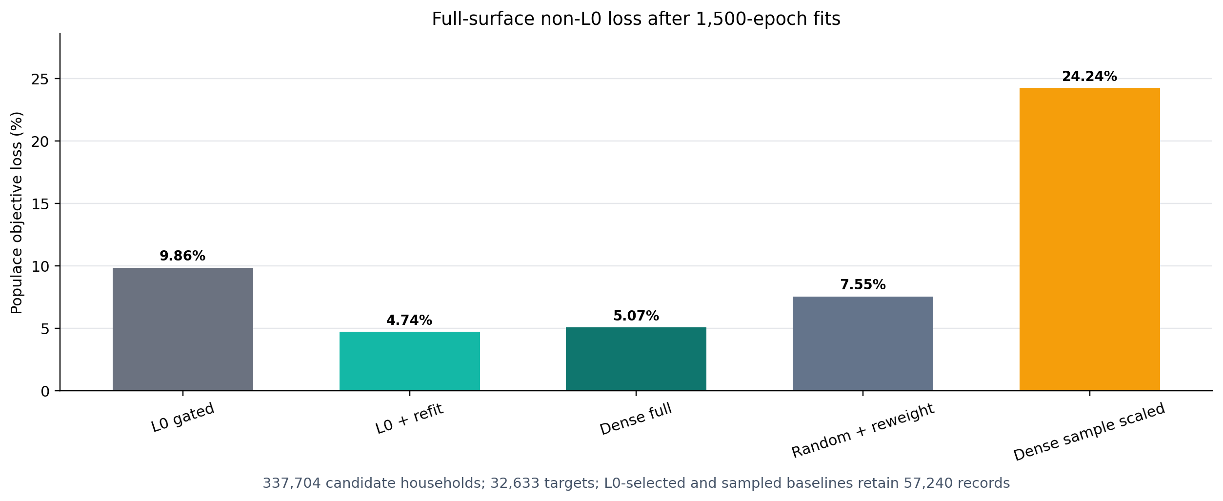
Figure 2 is the headline result. On the current three-year ASEC support file, the normalized \(L_0\) penalty selects 57,240 of 337,704 candidate households, or 17.0% of the candidate universe. The raw gated \(L_0\) weights are not the right publication weights: scored after thresholding, they reach a Populace objective loss of 9.86%. Removing the gates and refitting ordinary calibration weights on exactly the selected records lowers that loss to 4.74%. A dense no-\(L_0\) calibration using all 337,704 records and the same 1,500-epoch optimizer budget reaches 5.07%. A random subset of the same size as the \(L_0\) support, followed by the same 1,500-epoch gradient reweighting, reaches 7.55%. A random subset of the dense calibrated weights, scaled back to the dense total but not refit, reaches 24.24%.
The practical interpretation is that the \(L_0\) selector is doing useful support-selection work, but the post-\(L_0\) refit is essential. The selected support gives a lower finite-budget optimizer loss than the full dense run at 1,500 epochs and fits the full target surface much more closely than a random support of the same size. This should not be read as a claim that the dense feasible set is worse: the dense no-\(L_0\) loss is still declining at the end of the 1,500-epoch budget. The defensible claim is that this \(L_0\) support gives a better sparse support and a faster route to low loss under the completed optimizer budget. The current evidence should still be read as a single fixed-penalty probe, not as proof that this exact penalty is optimal: the next sweep needs to trace the normalized penalty across multiple retained counts and concentration settings.
Table [tab:sampling_comparison] reports the same comparison with raw ARE and weight diagnostics. The median ARE gives a different view from the capped objective: dense no-\(L_0\) has the lowest median ARE (0.56%), while the post-\(L_0\) refit is close (0.89%) and has the lowest capped Populace loss. Random + reweight has 6.70% median ARE, raw gated \(L_0\) has 11.66%, and the dense random scaled sample has 55.24%. The mean ARE remains much larger because a small tail of difficult IRS targets can have very large relative misses even when the capped Populace loss is low.
The \(L_0\) run uses normalized penalty share 0.8, equivalent to raw \(\lambda_{L_0}=2.37\times 10^{-6}\). Dense no-\(L_0\) is still declining at epoch 1,500, so its row is an epoch-matched finite-optimization baseline rather than a convergence certificate.
Table [tab:paired_comparison] expresses the comparison on the headline loss scale. Relative to dense no-\(L_0\), the post-\(L_0\) refit lowers the completed-run Populace objective by 6.4%. Relative to random + reweight, it lowers the objective by 37.2%. Relative to the raw gated \(L_0\) weights, it lowers the objective by 51.9%. The comparison isolates the value of the support and the refit: keeping dense weights on a random retained set and merely scaling them back to total mass performs poorly, so a sparse file still needs a reweighting step.
This table is descriptive because the current matched full-surface run uses one seed and one normalized \(L_0\) penalty. Dense no-\(L_0\), the post-\(L_0\) refit, and random + reweight all use 1,500 optimizer epochs, but dense no-\(L_0\) is still slowly declining at the end of that budget.
The normalized penalty gives a usable size control in this probe. We parameterize the sparsity price as a share of the mean calibration loss, \(\lambda_{\mathrm{share}}\sum_i\bar{z}_i/n\), rather than as an unscaled raw coefficient. With \(\lambda_{\mathrm{share}}=0.8\), the optimizer retained 57,240 records. This scaling matters operationally: the same raw coefficient has very different meanings when the candidate universe changes from tens of thousands to hundreds of thousands of records.
The selected support is more concentrated than the full dense calibration but better conditioned than the matched random sparse baselines. Dense no-\(L_0\) has an effective sample size of 5,970 and a maximum weight of 579,298. The post-\(L_0\) refit has ESS 4,726 and maximum weight 913,836. Random + reweight has lower ESS, 2,480, and a higher maximum weight, 1,163,939; the dense random scaled sample is worse again, with ESS 981 and maximum weight 2,176,121. The raw gated \(L_0\) weights have higher ESS, 6,879, but worse target fit, which is why the refit is the publishable sparse variant.
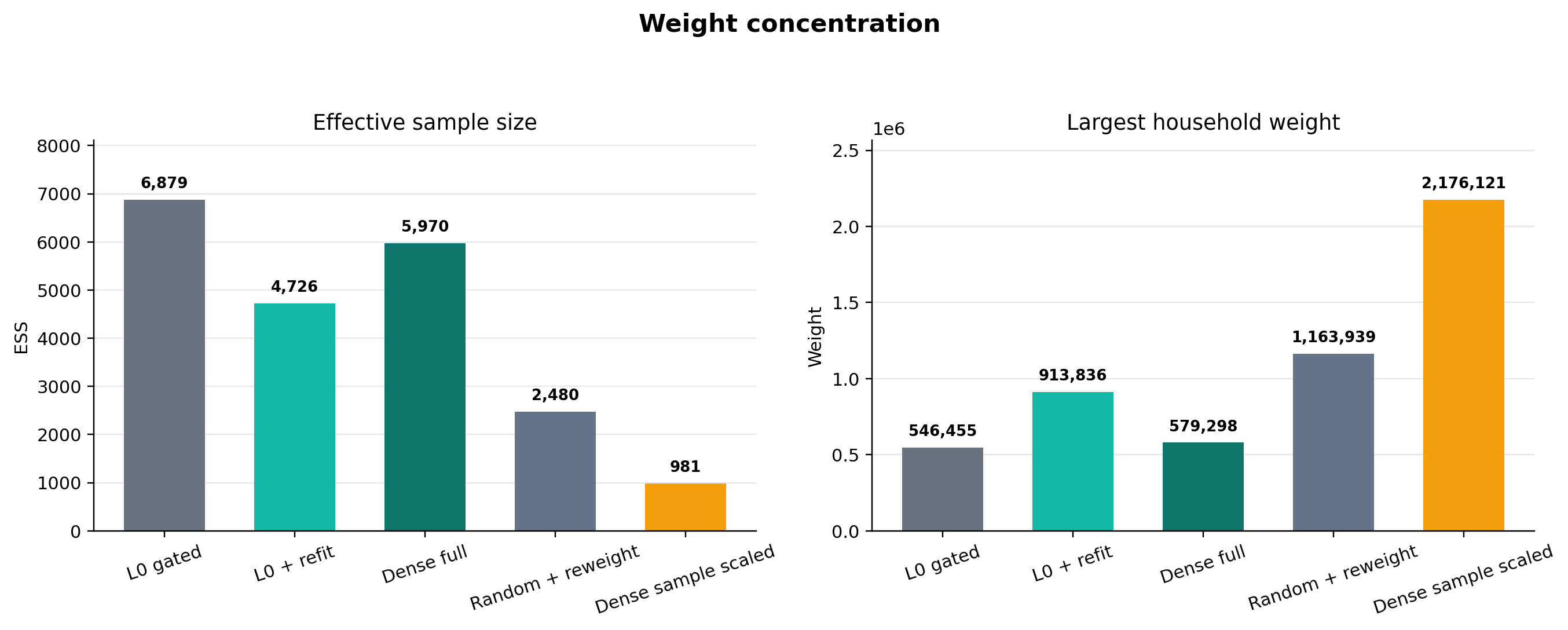
Table 4 breaks the post-\(L_0\) refit diagnostics down by geography. The fit is strongest at the state level, where median ARE is 0.31%, followed by national targets at 1.30% and district targets at 1.48%. District targets are the intended stress test for the method: they are the largest part of the target surface, and they are the reason Populace needs to build a large candidate universe before pruning it.
| Geographic level | Targets | Median ARE (%) | Mean ARE (%) | Max ARE (%) |
|---|---|---|---|---|
| National | 478 | 1.30 | 20.12 | 557.29 |
| State | 7,815 | 0.31 | 86.36 | 122,712.20 |
| Congressional district | 24,340 | 1.48 | 85.29 | 162,495.93 |
| All scored targets | 32,633 | 0.89 | 84.64 | 162,495.93 |
Raw ARE is undefined for 26 IRS SOI national targets where both target and achieved values are zero; those rows are included in the target count and the Populace loss but omitted from the raw ARE summary.
The Populace objective is the headline score because it is capped and target weighted; raw ARE summaries are supplemental. In the matched probe, raw ARE is defined for 32,607 of the 32,633 scored targets. The remaining 26 rows are IRS SOI national targets with both target and achieved values equal to zero, so they are omitted from raw relative-error summaries but do not affect the capped loss. Among the defined rows, the post-\(L_0\) refit has a 0.89% median ARE and an 84.64% mean ARE. The gap between the median and the mean is the reason the paper leads with the Populace loss and reports raw ARE only as a diagnostic.
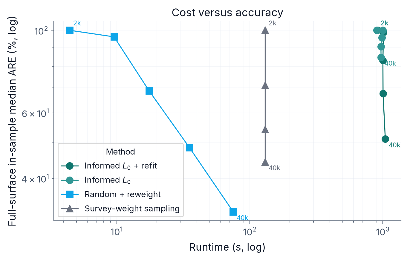
The matched probe took 39.4 minutes for the \(L_0\) selection run. The post-\(L_0\) refit then added about 9.5 minutes, for a combined 48.9 minutes reported in the artifact. Dense no-\(L_0\) took 38.7 minutes for 1,500 epochs, random + reweight took 7.3 minutes, and the dense random scaled sample required no extra optimization beyond the dense fit. The selector is therefore computationally expensive, and the dense run is still slowly declining at the endpoint. The accuracy gain over dense and random + reweight is large enough in this probe to justify a broader normalized-penalty sweep, but not enough to skip the next robustness work: more penalties, longer dense convergence checks, more candidate-support regimes, and concentration controls. Figure 4 in Appendix 13 plots wall-clock runtime against accuracy across requested record budgets as a supplemental cost diagnostic from the earlier budget sweep.
The matched full-surface probe supports the central version of the \(L_0\) hypothesis, with an important qualification. If the claim is that the raw gated weights returned by the joint \(L_0\) optimization should be the final publication weights, the evidence does not support it: the thresholded gated weights have a 9.86% Populace loss. If the claim is instead that target-informed gates can select a useful support for ordinary calibration, the evidence is positive. After the gates choose 57,240 records, an ordinary calibration refit on that support reaches 4.74% loss, below the dense no-\(L_0\) calibration and the matched sampling baselines reported in Section 5.
That distinction is useful. It separates selection from weighting. The Hard Concrete gates appear valuable as a way to decide which records survive, but the final dataset should be produced by a post-selection calibration refit rather than by directly publishing the stochastic-gate weights. This is also consistent with how the method would be used operationally: choose a sparsity penalty, use \(L_0\) to prune a deliberately overbuilt support, then run the standard Populace calibrator on the retained records. The slight edge over dense no-\(L_0\) at 1,500 epochs should be read as a finite-optimization result: the dense run is still declining, so a longer dense convergence check remains necessary.
The normalized sparsity scale is necessary. A raw \(\lambda_{L_0}\) cannot be interpreted across candidate universes of different sizes: the same coefficient can be mild on a small support and overwhelming on a larger one. Expressing the penalty as \(\lambda_{\mathrm{share}}\sum_i\bar{z}_i/n\) gives a dimensionless control, and \(\lambda_{\mathrm{share}}=0.8\) selected a meaningful sparse support in the three-year ASEC build. This does not remove the need for a sweep, but it gives the sweep a stable axis.
The concentration diagnostics are also encouraging in this probe. Dense no-\(L_0\) has the highest ESS among the publishable fits, but it retains every record. Among the sparse 57,240-record fits, the post-\(L_0\) refit has higher ESS and lower maximum weight than the matched random + reweight baseline, while fitting the targets more closely. That does not prove the concentration issue is solved: different penalties, seeds, and candidate-support regimes may move the frontier. But it means the current positive result is not bought by making the random baseline look better-conditioned.
The current result is a matched full-surface probe, not a completed frontier. It uses one normalized sparsity penalty and one seed. The next version should sweep \(\lambda_{\mathrm{share}}\) across multiple retained counts and run dense no-\(L_0\) to an explicit stopping rule; replicating the key points across seeds would harden the comparison but is secondary to mapping the penalty frontier. The present result is enough to justify that sweep because it shows a clear separation from random + reweight at one large, realistic support size and a small finite-budget edge over dense no-\(L_0\).
The target set is the current materialized Populace surface, not a hand-pruned paper subset. It is still conditional on what the source facts and current PolicyEngine variables can materialize, and the empirical claims are tied to the exact targets in each run’s manifest. A different Ledger surface, PolicyEngine version, materialization registry, or production weighting scheme could change the comparison.
The random + reweight baseline is strong because it uses the same gradient calibrator as the post-\(L_0\) refit after drawing the subset. It is therefore not a straw baseline: it is the practical reduce-first, calibrate-after workflow an analyst could run today. The dense random scaled sample answers a different question: whether one can dense-calibrate once, keep a random subset of the dense weights, scale the retained mass back up, and avoid refitting. On this surface that is not competitive. A fuller paper should still add the probability-proportional-to-size calibrate-then-sample comparator from the literature and classical calibration comparators on target subsets where they are well-defined.
The raw mean ARE remains tail-sensitive even when the Populace loss is low. The paper therefore leads with the capped, target-weighted Populace objective loss and reports median/mean ARE as supplemental diagnostics. The raw median is useful for typical target fit; the raw mean is useful for finding the tail.
Informed \(L_0\) is more expensive than the random baseline because it first has to learn the support. Dense no-\(L_0\) is also expensive because it keeps all records active. In this matched probe, \(L_0\) selection plus refit takes longer than the 1,500-epoch dense no-\(L_0\) run but returns a sparse 57,240-record support with lower completed-run loss. That cost is only worth paying if the selected subset is materially better, or if the method delivers an operational constraint that the baselines cannot. A production build still needs a penalty schedule, dense convergence checks, and checkpointing that make the sweep reliable.
The data engineering here is specific to the United States, but the question is general. Many microsimulation projects combine sources into a candidate dataset larger than they can ship, and then have to reduce it. This run shows that target-informed sampling can be evaluated on the real production loss and target surface. It also clarifies the benchmark: the method should be judged by whether the selected support, after ordinary refit, beats random + reweight and other practical baselines at the same retained count.
This study moves the proof of concept onto Populace’s current full target surface, including congressional-district targets. The next empirical step is to turn the matched probe into a frontier by sweeping the normalized sparsity share across retained counts. Holdout panels should remain separate robustness checks that ask narrower questions: which target families or geographies generalize when withheld, which targets dominate the loss, and how sensitive the result is to the production target weights and cap.
A related thread varies the penalties the headline run deliberately
holds fixed. The reported experiments set \(\lambda_{L_2}=0\) and leave the weight cap
off, so the comparison isolates the effect of the \(L_0\) gates on sparsification; this leaves
the concentration controls as a clean axis to study on their own. Three
experiments follow. First, evaluate the convex \(L_1\) selector of Section 2.6 head-to-head with \(L_0\) on the same surface: because a single
\(L_1\) penalty couples how many
records survive with how much the survivors shrink, we expect it to be a
weaker selector than the \(L_0\) gates,
and running it would show whether that coupling actually costs it.
Second, sweep the soft concentration penalty \(\lambda_{L_2}\) and the hard
max_weight_ratio cap against \(\lambda_{L_0}\). Third, use that sweep to
trace the effective-sample-size against accuracy trade-off, quantifying
how much calibration fit a build gives up to bound weight
concentration.
A second thread is the build-large-then-prune regime the controls are designed for, in which a pipeline assembles a candidate universe far larger than it can ship—hundreds of thousands or millions of records rather than a compact survey file—and prunes it to a deployable budget under the calibration targets. The current three-year support file is a step in that direction. More aggressive support expansion is where target-informed selection has its clearest opportunity to justify its cost: a random draw from a tight budget is least likely to span a demanding target system, so a selector trained on the targets has the most to add.
The full-surface design also clarifies which classical comparators are worth adding. Survey-weight (probability-proportional-to-size) sampling is the natural calibrate-then-reduce counterpart to random + reweight and belongs in the next frontier as a literature comparator, with the caveat that it selects records by the population mass they represent rather than by their fit to the targets. Raking, GREG, balanced sampling, and combinatorial optimization remain relevant reference methods, but not all are natural baselines for a heterogeneous 32,633-target fiscal surface. The appropriate next comparison is on the simpler categorical-margin subsets where their assumptions hold cleanly, in the spirit of Tanton et al. (2014)’s comparison of generalized regression with combinatorial optimisation for small-area reweighting, while the production frontier continues to use the Populace loss over the complete surface.
This paper studies \(L_0\) regularization as a way to subsample a large microsimulation dataset down to a usable size. The problem arises because a pipeline built for fidelity combines many sources and adds record-level geographic variation, which produces more candidate records than a deployable dataset can hold. The reduction to a fixed budget is a sampling choice, and the paper treats it as one.
The method uses Hard Concrete gates to select records and fit their weights in one optimization, with selection driven by the calibration targets. The current full-surface probe shows that the gates are most useful as a support selector. On the full Populace target surface, a normalized \(L_0\) penalty retained 57,240 of 337,704 candidate household records. Publishing the raw gated weights would leave too much loss, but refitting ordinary calibration weights on the selected support reduced the Populace objective to 4.74%. The same 1,500-epoch budget gives 5.07% for dense no-\(L_0\) calibration, 7.55% for a matched random support followed by the same reweighting, and 24.24% for a random sample of dense calibrated weights scaled back to total mass without refitting.
The result is not the final frontier; it is the first presentable full-surface signal. It justifies a broader sweep over normalized sparsity penalties, seeds, and concentration controls, with dense calibration run to a stopping rule and survey-weight and classical calibration comparators from the literature added where they are appropriate. The contribution is therefore twofold: a target-informed sampling method that can select a sparse support with lower completed-run loss than the current random and dense baselines, and an open Populace pipeline that makes such support-selection experiments reproducible on the real production target surface.
All authors are affiliated with PolicyEngine, the nonprofit
organization that develops Populace and
the l0-python package evaluated in this paper. The authors
have no other competing interests.
This work was funded by Arnold Ventures.
The paper and experiment code are at https://github.com/PolicyEngine/l0-paper. The
construction and calibration pipeline is implemented in Populace, PolicyEngine’s microsimulation data
stack, open source at https://github.com/PolicyEngine/populace; earlier
prototype code in the archived microplex and
microplex-us repositories is retained only as a migration
reference. The administrative targets are source-backed facts from
PolicyEngine Ledger, open source at https://github.com/PolicyEngine/arch-data. The
l0-python PyTorch package that implements the Hard Concrete
optimizer is available at https://github.com/PolicyEngine/l0-python. The candidate
universe used here is a generated three-year pooled ASEC support
artifact from Populace commit
558e46c1, with base H5 SHA-256 beginning
ec290055; the target facts have SHA-256 beginning
82cd9e87. The current reproduction workflow relies on
public code and generated data artifacts.
The authors used Claude (Anthropic) and Codex (OpenAI) for code assistance and manuscript drafting. All technical content, methodology, and analysis were designed and validated by the authors.
This study calibrates to the full materialized target surface Populace currently constructs for the US fiscal
build. Every target is a source-backed fact from PolicyEngine Ledger
(PolicyEngine
2026a), the arch-data fact store that holds the
source publications and preserves the provenance of each published
value; Populace composes calibration targets from those facts. The
surface combines national, state, and congressional-district aggregates
across the major tax and transfer families (Table 5). It is reported here in full
so the empirical claims can be read against the exact target system used
rather than against a pipeline-wide inventory.
Table 5 lists each family with its
administrative source. The system holds 32,633 targets
across eleven families and three geographic levels: 24,340
congressional-district, 7,815 state, and 478 national
targets. The irs_soi family supplies 31,350 of
them (96%), so any error summary aggregated over all targets is
dominated by IRS income-tax aggregates.
| Family | Administrative source | Levels | Targets |
|---|---|---|---|
irs_soi |
IRS Statistics of Income: Historic Table 2 state totals and congressional-district tables | National, state, district | 31,350 |
census_pep |
Census Bureau annual state resident population estimates | National, state | 936 |
cms_medicaid |
CMS Medicaid and CHIP applications, eligibility, and enrollment reports | National, state | 102 |
cms_aca |
CMS open-enrollment-period state-level public use file | State | 102 |
usda_snap |
USDA FNS SNAP monthly state participation and benefit summaries | National, state | 52 |
census_stc |
Census Bureau State Tax Collections (STC), item T40 individual income taxes | State | 44 |
hhs_acf_tanf |
HHS ACF federal TANF and state MOE financial data | National, state | 30 |
ssa_supplement |
SSA Annual Statistical Supplement, OASDI beneficiaries and benefits | National | 6 |
jct |
JCT estimates of federal tax expenditures | National | 5 |
cbo |
CBO revenue projections by category | National | 5 |
cms_medicare |
CMS Medicare Trustees Report | National | 1 |
| Total | 32,633 |
Table 6 lists the hyperparameters of the \(L_0\) optimization with their roles. The gate parameters follow the Hard Concrete construction of Louizos et al. (2018). The sparsity penalty \(\lambda_{L_0}\) and the epoch count are set per build to reach a target dataset size and are reported with each run.
| Parameter | Value | Role |
|---|---|---|
| Gate temperature \(\beta\) | 0.25 | Sharpness of the 0/1 gate transition |
| Left stretch \(\gamma\) | \(-0.1\) | Enables exact-zero gates after clipping |
| Right stretch \(\zeta\) | 1.1 | Enables exact-one gates after clipping |
| Initial keep probability | 0.8 | Records start mostly active while leaving room for the sparsity penalty to close gates |
| Weight jitter SD | 0.05 | Log-space noise on weights at initialization |
| Logit jitter SD | 0.01 | Log-space noise on gate logits at initialization |
| Learning rate | 0.02 | Adam optimizer step size |
| Epochs | 1,500 | Training iterations in the reported fixed-penalty probe |
| Target loss cap \(c\) | 1 | Caps a single target’s contribution to \(\mathcal{L}_{\text{cal}}\); the runs reported here use Populace’s production US-fiscal value \(c=1\) |
| \(\lambda_{\mathrm{share}}\) | 0.8 | Normalized sparsity share in \(\lambda_{\mathrm{share}}\sum_i\bar{z}_i/n\); raw \(\lambda_{L_0}=2.37\times10^{-6}\) for 337,704 records |
| \(\lambda_{L_2}\) | \(0\) | Soft concentration penalty on \((w_i/w_{0,i})^2\) (mean over records); held at zero in the reported full-surface run |
| Budget bisection steps | None | The reported full-surface probe uses one fixed normalized penalty; a future frontier should sweep this value |
max_weight_ratio |
None (uncapped) | Hard per-record weight cap: \(w_i \leq \text{ratio}\times w_{0,i}\), clamped each step |
Algorithm [alg:l0] presents the \(L_0\)-regularized calibration procedure.
Calibration matrix \(\mathbf{M} \in
\mathbb{R}^{m \times n}\), targets \(\mathbf{t} \in \mathbb{R}^m\), initial
weights \(\mathbf{w}_0 \in
\mathbb{R}^n\), per-target loss weights \(\boldsymbol{\omega} \in \mathbb{R}^m\)
Hyperparameters: \(\lambda_{L_0}\),
\(\lambda_{L_2}\), weight cap \(r\) (max_weight_ratio; \(\infty\) if uncapped), \(\beta\), \(\gamma\), \(\zeta\), learning rate \(\eta\), epochs \(E\) Calibrated sparse weight vector \(\hat{\mathbf{w}} \in \mathbb{R}^n\)
Initialize \(\log w_i \gets \log w_{0,i} + \mathcal{N}(0, 0.05^2)\) for all \(i\) Initialize \(\log \alpha_i \gets \text{logit}(0.8) + \mathcal{N}(0, 0.01^2)\) for all \(i\) Initialize Adam optimizer with parameters \(\{\log w_i, \log \alpha_i\}\) and learning rate \(\eta\)
Sample Hard Concrete gates (training): \(u_i \sim \text{Uniform}(\epsilon, 1-\epsilon)\) \(s_i \gets \sigma\!\left(\frac{\log u_i - \log(1-u_i) + \log \alpha_i}{\beta}\right)\) \(\bar{s}_i \gets s_i(\zeta - \gamma) + \gamma\) \(z_i \gets \min(1, \max(0, \bar{s}_i))\) \(w_i^{\text{eff}} \gets \exp(\log w_i) \cdot z_i\) for all \(i\) \(\hat{t}_j \gets \sum_i M_{ji} \cdot w_i^{\text{eff}}\) for all \(j\) \(\mathcal{L}_{\text{cal}} \gets \dfrac{\sum_{j=1}^{m}\omega_j\,\min\!\left(\left|\frac{\hat{t}_j - t_j}{s_j}\right|, c\right)}{\sum_{j=1}^{m}\omega_j}\) \(\mathcal{L}_{L_0} \gets \sum_{i=1}^{n} \sigma\!\left(\log \alpha_i - \beta \log \frac{-\gamma}{\zeta}\right)\) \(\mathcal{L}_{L_2} \gets \frac{1}{n}\sum_{i=1}^{n}\left(\frac{\exp(\log w_i)}{w_{0,i}}\right)^2\) \(\mathcal{L} \gets \mathcal{L}_{\text{cal}} + \lambda_{L_0} \mathcal{L}_{L_0} + \lambda_{L_2} \mathcal{L}_{L_2}\) Backpropagate \(\nabla_{\log w, \log \alpha} \mathcal{L}\) Adam step Clamp \(\log w_i \gets \min\!\left(\log w_i,\; \log(r \cdot w_{0,i})\right)\) for all \(i\)
Deterministic inference: \(z_i^{\text{det}} \gets \min\!\left(1, \max\!\left(0,\; \sigma(\log \alpha_i)(\zeta - \gamma) + \gamma\right)\right)\) \(\hat{w}_i \gets \exp(\log w_i) \cdot z_i^{\text{det}}\) \(\hat{\mathbf{w}}\)
After optimization the fitted weight vector is mapped back to record form and used to assemble the deployable dataset. The assembly step keeps the active records, reconstructs their person and tax-unit memberships, derives geography from the stored assignment, and recomputes geography-dependent quantities. Two details matter for fidelity. Geography is derived from the same assignment used to build the calibration matrix, so the assembled dataset matches the universe the optimizer saw. Take-up draws are regenerated with the same deterministic seeds used during matrix construction, so take-up-dependent targets stay consistent between the calibration problem and the assembled dataset.
Figure 4 is retained as a supplemental cost diagnostic from the earlier budget sweep. The matched full-surface probe’s current runtimes are reported in Section 5: dense no-\(L_0\) took 38.7 minutes for 1,500 epochs, \(L_0\) selection plus refit took 48.9 minutes combined, and random + reweight took 7.3 minutes.
PolicyEngine. Corresponding author: maria@policyengine.org↩︎